How do we price risk?

Source

Our project examines the predictors of interest rates in an online peer-to-peer lending marketplace.

Using data from the Lending Club, we examine 887,379 unique loans issued between 2007 and 2016 (source).

Basic summary stats

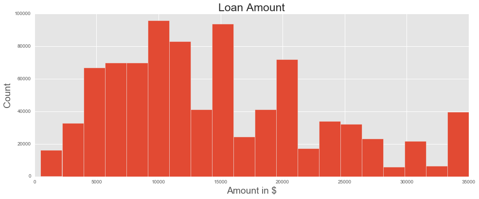
The average loan amount is $14,755, with most loans (67%) still being active, a sizable minority (23%) already paid off, and the remaining in various states of tardiness, default, and charge-off. (Charge-off occurs when a creditor declares that a debtor is no longer able to pay the loan; usually, this can happen after loan payments are six months behind schedule.)

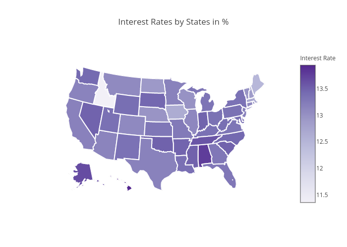
All borrowers are assigned a FICO score - something which should signal a borrower’s riskiness to potential creditors. Scores range from A (least risky) to G (most risky). Less than 10% of borrowers have scores below D - the majority are in the top three (least risky) ranges: A (17%), B (29%), and C (28%). Borrowers are then ‘priced’ according to their riskiness, and this is reflected in the interest rates. Indeed, while the average interest rate across all loans was 13%, this varies substantially by grade.

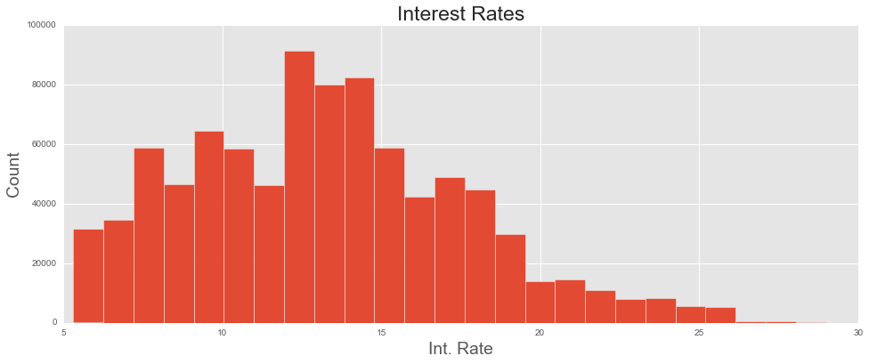
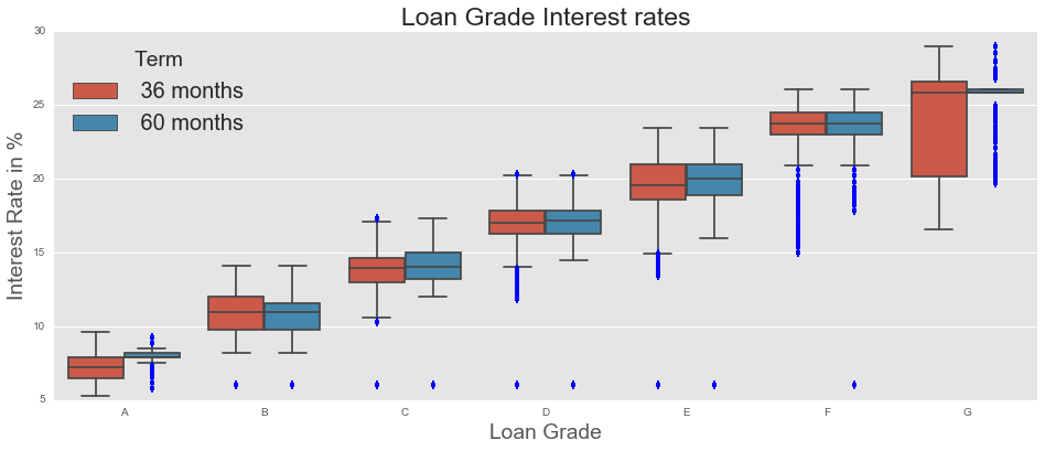
As expected, the interest rate is positively correlated with loan grade: as loans get riskier, borrowers must pay more to lenders to take on that risk.

A strategy forward

Interest rates are directly correlated with a borrower's grade, but that does not necessarily provide us with much useful information: both the interest rate and grade of a borrower are attempting to capture the same thing (riskiness). So a better question to ask is: what could predict a borrower’s riskiness? Possible predictors include individual-level characteristics which are measurable but may not be available in this dataset (education, employment status, social network, spending behavior), measurable and available in this dataset (debt-to-income ratio, purpose of loan), and difficult to measure altogether (risk tolerance, likelihood of exogenous income or spending shocks).

Considering information which is available in the Lending Club dataset: The majority of loans (59%) are used to consolidate debt. This becomes 82% if we include credit card payments. In other words, the majority of borrowers on Lending Club are borrowing in order to pay off other debt. This seems to imply that the Lending Club data is a selected sample, not necessarily representative of the entire population of borrowers. Indeed, Lending Club seems unlikely to be the first ‘port of call’ for borrowing; rather, we could speculate that most borrowers go to Lending Club when they are further along their debt journey.

The debt-to-income (DTI) ratio is 18% - meaning, the average LC borrower must spend around 18% of their monthly income on their other loans (excluding mortgages and the requested LC loan). In general, we can expect that borrowers with higher DTI ratio will have more difficulty in paying off their loan - a predictor for default, and also, perhaps, a predictor for higher interest rates. The DTI distributions also shift according to grade: with less risky borrowers having lower DTI ratios, on average, than more risky borrowers.

A baseline, and beyond

To begin our analysis, we created a set of baseline predictions. We conducted minimal data cleaning and examined a wide range of models (linear regression with Ridge and Lasso regularization terms, an AdaBoost model, random forests) - our best prediction attained an R² of around 56%. (As a reminder: R² measures the proportion of variance found in the data which the model can explain - the lower this measure is, the less your model 'explains' the variation we see in the real world.) An R² of 56% is reasonable as a baseline. With it, we could proceed with some confidence that the dataset contained, at least, a significant potential to predict.

Data: Preparing for the model

But how to improve from the baseline? Following the philosophy of GIGO - Garbage In, Garbage Out - we focused on feature engineering and surgical data cleaning.

We dealt with missing, non-numerical and categorical values. Furthermore, we moved our data cleaning out of Jupyter notebooks and into Python modules. This standardized our process, ensuring the raw data was processed in the same way across our machines and our work was consistently and version controlled. See below for an example method, clean_data(dataset), from our make_dataset.py module. This method provided the base cleaning, removing outliers and so forth.

Missing data was imputed following exploratory data analysis which identified that, on the whole, imputing to zero was the most appropriate option.

As a third step, we prepared two functions: one for a richer model, and one for a simpler improvement of the baseline. Given the deadline of this project (Dec 14, 2016), we chose to submit the simpler model: eliminating the more computationally-intensive feature engineering around string variables and geo-coding economic information. While conducting deeper text analysis and an economic analysis of states/zip codes might have provided improved predictions, it was decided that the marginal added value of these columns (e.g. the average income of each state) was unlikely to significantly outweigh the marginal computational cost of producing these features. Given this, we ran the simple_dataset(dataset) method in our data cleaning Python modules (see below).

The full code (including Jupyter notebooks for analysis and Python modules for data cleaning) can be found here.

Train, test split

We can use past years as predictors of future years. One challenge with this approach is that we confound time-sensitive trends (for example, global economic shocks to interest rates - such as the financial crisis of 2008, or the growth of Lending Club to broader markets of debtors) with differences related to time-insensitive factors (such as a debtor's riskiness). To account for this, we cross-validated sets within time blocks, and used each previous year to predict the following year. In general, this did not yield very good results.

As we can see, restricting ourselves to a year-specific model limits our predictive power. Following this, we opted to use the entire dataset and run a standard training/test split on it instead. This assumes that, over the course of Lending Club's history (which includes, for example, the financial crisis of 2008), we have sufficient sample size to 'smooth out' time-specific shocks.

Fitting the model

The ultimate model we chose was a Random Forest Regressor. This was mostly due to the Random Forest behaving as a strong, non-parametric choice for large datasets. It allowed us to approach the problem without making underlying assumptions about the shape of the data. This was especially beneficial given that, while we have some domain knowledge, we would require more time to conduct a deeper literature review around peer-to-peer lending markets. The Random Forest allowed us to 'throw everything in' and see how a (relatively computationally intense) algorithm identifies boundaries. To compare, we also looked at the Ridge regression and AdaBoost algorithm from the baseline set. In this way, we could likewise evaluate the improvement generated from proper data cleaning.

We limited the number of decision trees in our Random Forest; this was selected to limit overfitting and restrict computational time. Likewise, we follow the advice of Breiman and Cutler in selecting the maximum number of features per tree to be the square root of the total number of features. We did not tune further.

In general, the Random Forest - coupled with the 'freshly cleaned' data - outperformed both the AdaBoost regression (by a significant amount), as well as the regularized linear regression.

Model	Cross-validated R2
Ridge Regression	0.67
Ada Boost Regression	0.28
Random Forest Regression	0.83

Examining the relative feature importances (how often and how 'fundamental' each feature is to each individual decision tree's splits), we see that the most important features in the Random Forest were: total interest received, the loan's term length (term_60 months), the monthly payment amounts (installment), and the amount of credit a borrower is using relative to their total amount (revol_util).

Feature	Importance
total_rec_int	0.139426
term_ 36 months	0.130110
installment	0.073718
revol_util	0.059305
total_rec_prncp	0.053989

Of course, to call these features 'predictive' would be to conflate correlation with causation. This is a core philsophical 'blind spot' of data science: it has a singular focus on correlation, and using increasingly large datasets to generate hyper-precise predictions based on comprehensive correlations. The problems arise when the predictive features (i.e. highly correlative terms) are no longer in the dataset: without an underlying theory to explain predictions (for example, an economic theory model of risk-taking and lending behavior), or without - at least - an empirical analysis of causal factors, we are left with little.

In this case, we have found that our model would be able to 'predict' interest rates if given a blind dataset with the features listed above. However those features are, by definition, concurrent: at the same time that monthly payment plans are set, so is the interest rate. Does the monthly payment 'predict' the interest rate? Yes. But does it cause it? Clearly, no. Similarly for the other predictive features: they are indicative of what an interest rate would be, if it was the missing piece. But they do not predict the interest rate.

So how could we predict interest rates, in the sense of identifying causal factors? This is where the interesting, more computationally intensive feature engineering could help. Perhaps certain zip codes contain socio-economic information and, for example, poorer zip codes lead to higher interest rates. Perhaps frequent misspellings in the text fields of a Lending Club form lead peer-to-peer lenders to raise the 'minimum acceptable interest rate'. And perhaps, finally, we can dig into the economic theory of lending markets to find other hypotheses of causal factors to improve our predictions.